Example Akuna Capital Interview Questions

Options are financial derivatives that give the holder the right, but not the obligation, to buy or sell an underlying asset at a predetermined price, known as the strike price, within a specified period. There are two primary types of options: American options and European options. The main difference between these two types of options lies in the timing of when they can be exercised.

American Options
An American option can be exercised at any time up until the expiration date. This flexibility allows the holder to capitalize on favorable market movements at any point during the option's life. For example, if the price of the underlying asset moves significantly in favor of the option holder before the expiration date, the holder can exercise the option to capture the profit immediately.

The ability to exercise at any time provides a strategic advantage, particularly in volatile markets or when the underlying asset pays dividends. For instance, an investor holding an American call option on a dividend-paying stock might choose to exercise the option just before the ex-dividend date to receive the dividend payment.

European Options
In contrast, a European option can only be exercised at the expiration date, not before. This restriction means that the holder must wait until the expiration date to exercise the option, regardless of any favorable movements in the price of the underlying asset during the option's life. As a result, European options typically trade at a discount compared to American options, all else being equal, because they offer less flexibility to the option holder.

European options are often used in markets where the underlying asset is less volatile and the need for early exercise is minimal. The pricing of European options is generally simpler due to the fixed exercise date, making them a popular choice for certain financial models and strategies.

The pricing of American and European options also differs due to the exercise flexibility. The Black-Scholes model, for instance, is primarily used for pricing European options and assumes constant volatility and a constant interest rate. American options, however, require more complex models, such as the binomial options pricing model, which can accommodate the possibility of early exercise.

This is a pretty straightforward Markov chain problem. There are 4 states. The transition graph is given in Figure 1.

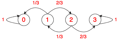
The problem starts at state 1. As has been explained in the lessons of this course, we use the following equation:
\begin{equation}
s_1 = \sum_{i=0}^{3}p_{1,i}s_i
\end{equation} \begin{equation}
s_2 = \sum_{i=0}^{3}p_{2,i}s_i
\end{equation} Furthermore, $s_0=0$ and $s_3=1$. Then we have
\begin{equation}
s_1 = \frac{1}{3}*0 + \frac{2}{3} * s_2
\end{equation} \begin{equation}
s_2 = \frac{1}{3}* s_1 + \frac{2}{3} * 1
\end{equation} Solving these equations gives us $s_1=4/7$ and $s_2=6/7$. So, starting with 1 dollar, player A has a 4/7 chance of winning.

Proof
If we substitute Equation 4 in Equation 3, we have

\begin{equation}
s_1 = \frac{1}{3}*0 + \frac{2}{3} * (\frac{1}{3}* s_1 + \frac{2}{3} * 1)
\end{equation} \begin{equation}
s_1 = \frac{2}{9} * s_1 + \frac{4}{9}
\end{equation}  \begin{equation}
\frac{7}{9} * s_1 =  \frac{4}{9}
\end{equation}  \begin{equation}
s_1 =  \frac{4}{9} / \frac{7}{9} = \frac{4}{7}
\end{equation}

This is called the coupon collector problem. For a fair n-sided die, the expected number of attempts needed to get all n values is \begin{equation}
n \Sigma_{k=1}^n \frac{1}{k}
\end{equation} which, for large n is approximately n log n.

The time until the first result appears is 1. After that, the random time until a second (different) result appears is geometrically distributed with parameter of success 5/6, hence with mean 6/5 (recall that the mean of a geometrically distributed random variable is the inverse of its parameter). After that, the random time until a third (different) result appears is geometrically distributed with parameter of success 4/6, hence with mean 6/4. And so on, until the random time of appearance of the last and sixth result, which is geometrically distributed with parameter of success 1/6, hence with mean 6/1. This shows that the mean total time to get all six results is \begin{equation}
6 \Sigma_{k=1}^6 \frac{1}{k} = \frac{147}{10} = 14.7
\end{equation}

# Implementing the Longest Common Subsequence (LCS) using Dynamic Programming

def find_lcs(seq1, seq2):

    n = len(seq1)

    m = len(seq2)

    

    # Initialize a DP table with zeros

    dp = [[0] * (m + 1) for _ in range(n + 1)]

    

    # DP step: fill in the table

    for i in range(1, n + 1):

        for j in range(1, m + 1):

            if seq1[i-1] == seq2[j-1]:

                dp[i][j] = dp[i-1][j-1] + 1

            else:

                dp[i][j] = max(dp[i-1][j], dp[i][j-1])

    

    # Reconstruct the LCS

    lcs = []

    i, j = n, m

    while i > 0 and j > 0:

        if seq1[i-1] == seq2[j-1]:

            lcs.append(seq1[i-1])

            i -= 1

            j -= 1

        elif dp[i-1][j] > dp[i][j-1]:

            i -= 1

        else:

            j -= 1

    

    return lcs[::-1]  # Reverse the LCS to get it in the correct order



# Test the function

seq1 = [1, 2, 3, 4, 5]

seq2 = [6, 7, 1, 2, 8]

print(find_lcs(seq1, seq2))  # Should return [1, 2]